Funded by the European Union and the European Research Council ADDI — Advancing Digital Democratic Innovation

EDDY 2026

Efficient Elicitation of
Collective Disagreements

Mohamed Ouaguenouni1, Felipe Garrido-Lucero1, Umberto Grandi1, César Hidalgo2,3,4, Magdalena Tydrichova5

1. IRIT, Université Toulouse Capitole, Toulouse, France
2. Center for Collective Learning, IAST, Toulouse School of Economics, France
3. Center for Collective Learning, CIAS, Corvinus University of Budapest, Hungary
4. AMBS, University of Manchester, UK   5. Centrale Supélec, Paris Saclay, France

The setting

Alternatives, people, and preferences

We have \(m\) alternatives: \(\mathcal A=\{a_1,\ldots,a_m\}\).

a₁a₂a₃⋯aₘ

People can compare them using a binary relation \(\succ\).

\(A\succ B\) means A is better than B
for that person.

We model each person’s preferences as a strict, complete, transitive ranking.

Choosing a winner

Gentle Warmup

Computational social choice often asks: which alternative should win?

One way is to give points according to rank. Borda score

People’s rankings

1\(a_1\succ a_2\succ\cdots\succ a_m\)
2\(a_3\succ a_2\succ\cdots\succ a_m\)
\(\vdots\)
\(n\)\(a_2\succ a_1\succ\cdots\succ a_m\)

The Borda score

rank 1\(m\)
rank 2\(m-1\)
⋯
rank \(m\)\(1\)

An alternative’s rank distribution tells us how likely it is to be placed first, second, and so on.

$$B_n(a)=\frac1n\sum_{i=1}^{n}\bigl(m+1-r_i(a)\bigr).$$

Gentle Warmup · formal definitions

Profiles and rank distributions

Let $\mathcal A$ contain $m$ alternatives and $\mathcal L(\mathcal A)$ be their complete, strict rankings.

Definition · profile

A profile is a probability distribution over rankings:

$$\pi:\mathcal L(\mathcal A)\to[0,1],\qquad \sum_{\sigma\in\mathcal L(\mathcal A)}\pi(\sigma)=1.$$

$\pi(\sigma)$ is the probability that a randomly sampled person has ranking $\sigma$.

Definition · rank distribution

Let $r_\sigma(a)$ be the position of $a$ in ranking $\sigma$, with rank 1 best. Its rank distribution under $\pi$ is

$$q_a^\pi(j):=\Pr_{\sigma\sim\pi}[r_\sigma(a)=j]=\sum_{\sigma:\,r_\sigma(a)=j}\pi(\sigma),\qquad j=1,\ldots,m.$$

Thus $q_a^\pi(j)\ge0$ and $\sum_{j=1}^{m}q_a^\pi(j)=1$.

Three alternatives

Illustrative Exemple

To compute the Borda score

We don’t need the full profile

Pairwise proportions: \(p_{ab}=\Pr_{\sigma\sim\pi}[a\succ b]\).

$$B_\pi(a)=m+1-\mathbb E_{\sigma\sim\pi}[r_\sigma(a)]$$
ABC

Each arrow gives the probability that its source
is preferred to its target.

In the reverse direction: \(p_{ba}=1-p_{ab}\).

Understanding disagreement

Deliberation needs to know what is divisive

In digital democracy, we also want to structure deliberation around disagreements.

Uniform profile

\(\pi_U(\sigma)=\tfrac16\) for each of the six rankings.

Rank distribution of A

Different profiles. The same weighted tournament.
They are indistinguishable from pairwise proportions alone.

Technical branch · same margins

Why can no pairwise rule distinguish them?

PairPopulation UPopulation P

Every function whose input is only these three aggregate proportions receives the same input on U and P, so it must return the same output.

This does not say linked answers from the same voter are useless. Their joint pattern is precisely the information the separate margins discard.

What should we look at?

Pairwise proportions miss disagreement structure

Pairwise tournaments

Full profile?

Three measures from the literature

Some measures distinguish the two profiles

Several measures of divisiveness have been proposed in the literature.

Agreement index.Alcalde-Unzu & Vorsatz (2013) \(\displaystyle A(\pi)=\frac1{\binom m2}\sum_{\{x,y\}}\left|2p_{xy}-1\right|\)

Rank variance.Colley et al. (2023), §2.3 \(\displaystyle \operatorname{Var}_\pi(a)=\mathbb E_\pi[(r_a-\mathbb E_\pi[r_a])^2]\)

Divisiveness.Navarrete et al. (2024) \(\displaystyle \operatorname{Div}_\pi(a)=\frac1{m-1}\sum_{b\ne a}\left|B_\pi(a\mid a\succ b)-B_\pi(a\mid b\succ a)\right|\)

\(m=15\) alternatives · the focal alternative \(a\) is at an extreme in both opposed rankings.
Measure
\(\pi_{\rm IC}\) · uniform
\(\pi_{\rm AN}\) · antagonism
Agreement index\(0\)\(0\)
Rank variance\(\frac{56}{3}\)\(49\)
Divisiveness\(\frac{16}{3}\)\(14\)

“Rank variance and divisiveness see every disagreement structure
because they use the full profile.”

Are we sure?

A counterexample

Let’s suppose…

  • We have \(m\) alternatives, with one distinguished alternative \(a\).
  • We choose \(a\)’s rank using one of the distributions below.
  • We uniformly shuffle the other \(m-1\) alternatives into the remaining positions.

What do these profiles—with only \(a\)’s rank distribution changed—have in common?

Rank variance and divisiveness use the full profile.

What information are they using?

Technical branch · original five-profile construction

A changed focal histogram still defines a feasible profile

Draw rank \(R\sim w\) for \(a\), then uniformly permute the remaining labels over the vacant positions.

$$\pi_w(\sigma)=\frac{w_{r_\sigma(a)}}{(m-1)!}.$$

For these witnesses, \(\mu=(m+1)/2\) and \(v=(m^2-1)/12\).

$$\operatorname{Var}_\pi(a)=v,\qquad \operatorname{Div}_\pi(a)=\frac{4v}{m-1}=\frac{m+1}{3}.$$

“Uniform except for \(a\)” means a uniform shuffle conditional on \(a\)’s rank. Each other alternative’s marginal at rank \(j\) is \((1-w_j)/(m-1)\).

Technical branch · a separate exact seven-alternative witness

Another construction matches every entry through degree 3

Mean rank 4, variance 1.5, divisiveness 1 — and identical plurality data through degree 3.

Technical branch · seven-alternative witness · 1/2

The equality is stronger than matching mean and variance

Sample A’s rank from one of the displayed distributions. Conditional on that rank, place the other six alternatives uniformly in the remaining positions.

$$p_S(a)=\sum_{j=1}^{7}w_j\frac{\binom{7-j}{|S|-1}}{\binom{6}{|S|-1}}.$$

For pairs and triples this expression depends only on the first two rank moments. Symmetry fixes every other winner entry.

Therefore all degree-2 and degree-3 plurality entries agree exactly — not merely A’s histogram summaries.

Technical branch · seven-alternative witness · 2/2

The higher moments separate the three profiles

ProfileMeanVarianceSkewnessExcess kurtosis

The profiles remain indistinguishable through degree 3, then skewness and kurtosis reveal distinctions at higher resolution.

Higher moments add summaries; they do not reconstruct an arbitrary ranking distribution.

A framework for information

The plurality matrix records favorites in subsets

Definition · plurality cell

$$p_S^\pi(a):=\Pr_{\succ\sim\pi}\!\left[a\succ b\ \text{for every }b\in S\setminus\{a\}\right],\qquad a\in S\subseteq\mathcal A.$$

The probability that $a$ is favorite in $S$. The cell’s degree is $|S|$.

A profile on four alternatives

All other rankings have probability 0.

Degree 2 · pairsDegree 3 · triplesDegree 4 · all four
$S$ABCD

Each row sums to 1; — means $a\notin S$.

Technical branch · plurality matrix

One entry answers one subset question

$$p_S^{\pi}(a)=\Pr_{\succ\sim\pi}\!\left(a\text{ is ranked first within }S\right),\qquad a\in S.$$
  • Each row is indexed by a nonempty subset S.
  • Its entries sum to one: $\sum_{a\in S}p_S^{\pi}(a)=1$.
  • The row’s degree is $|S|$; degree 2 is pairwise information.
  • A measure’s level is the smallest cutoff that suffices in general.

A degree-k cutoff retains every row of degree 2 through k; it is not only the degree-k row.

How much information is enough?

The level is the smallest sufficient degree

Definition · level of a measure

A measure’s level is the minimal degree up to which we need the plurality matrix to express that measure.

Borda score and agreement index are level 2.

Rank variance and divisiveness are level 3.

Technical branch · formal definition of level

The level is a minimal sufficient cutoff

Definition · level of a measure

Write $P_{\le\ell}(\pi)=\bigl(p_S^\pi(a)\bigr)_{2\le |S|\le\ell,\ a\in S}$.

$$\operatorname{level}(D):=\min\!\left\{\ell:\ \exists f,\ \forall\pi,\quad D(\pi)=f\!\left(P_{\le\ell}(\pi)\right)\right\}.$$

Keep every degree up to $\ell$, not just degree $\ell$.

Technical branch · why triples appear · 1/2

Variance creates products of two pairwise indicators

$$X_b=\mathbf{1}\{a\succ b\},\qquad r_a=m-\sum_{b\ne a}X_b.$$
$$\mathbb{E}[X_b]=p_{\{a,b\}}(a),\qquad \mathbb{E}[X_bX_c]=p_{\{a,b,c\}}(a).$$

Expanding $\mathrm{Var}(r_a)$ introduces $X_bX_c$: the event that A beats both opponents in their triple.

The earlier U/P pair has identical pairwise data but different variance, proving pairwise insufficiency in general.

Technical branch · why triples appear · 2/2

Sufficiency and necessity answer different questions

Sufficiency

An explicit formula writes the measure using entries through degree 3.

Necessity in general

Two profiles agree through degree 2 but the measure changes.

Under additional structure, the hierarchy can collapse: for example, Plackett–Luce profiles or single-peaked preferences on a known common axis.

This does not say every real dataset needs degree 3, only that no degree-2 formula works for all unrestricted profiles.

The moment hierarchy

Can we go beyond level 3?

$$M_k^\pi(a)=\mathbb E_{\pi}\!\left[(r_a-\mu_a)^k\right],\qquad \mu_a=\mathbb E_{\pi}[r_a].$$

First moment → Borda
$B_\pi(a)=m+1-\mu_a$

Second central moment → rank variance
$M_2^\pi(a)=\operatorname{Var}_{\pi}(r_a)$

Proposition · moment–level correspondence

The $k$-th central moment has level $k+1$
for $k\ge2$ and $m\ge k+2$.

Compute it directly from the plurality matrix:

$$M_k^\pi(a)=(-1)^k\sum_{s=0}^{k}c_s(a)\underbrace{\sum_{\substack{S\subseteq\mathcal A\setminus\{a\}\\|S|=s}}p_{S\cup\{a\}}^\pi(a)}_{\text{degree }s+1\ \le\ k+1}.$$
$$c_s(a)=\sum_{j=0}^{s}(-1)^{s-j}\binom{s}{j}(j-q_a)^k,\qquad q_a=B_\pi(a)-1.$$

Convention: $p_{\{a\}}^\pi(a)=1$. Only degrees 2 through $k+1$ are needed.

Beyond spread

The same spread can hide different shapes

Asymmetry appears in the third central moment; sensitivity to extreme deviations appears in the fourth.

Skewness is level 4.   Excess kurtosis is level 5.

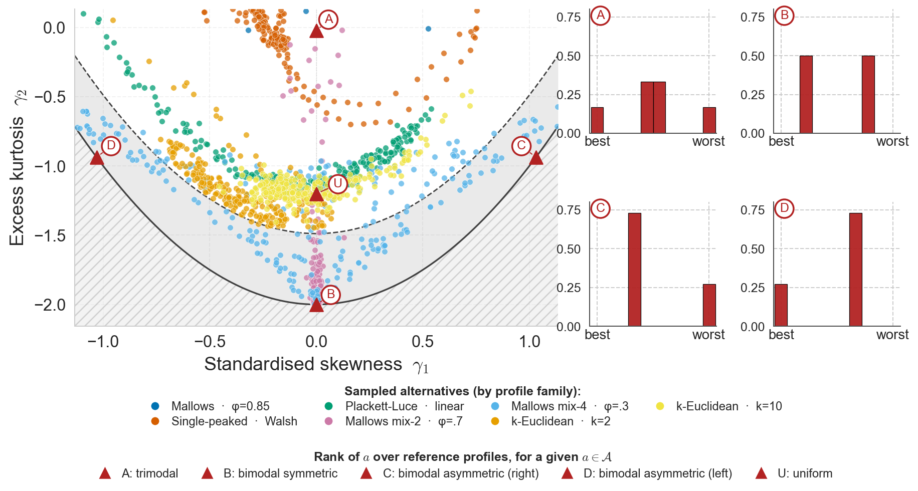
Skewness × kurtosis — the level-4 / level-5 plane

Original synthetic-data skewness–kurtosis figure

Open the interactive version ↓  ·  Full synthetic-data figure

Interactive · the moment plane

Synthetic models and real elections. Select an alternative to inspect its rank distribution.

Synthetic data · the complete figure

Original synthetic-data figure, with model clouds and reference rank distributions

Technical branch · moment plane · 1/2

Standardized moments require nonzero variance

$$\gamma_1=\frac{\mathbb{E}[(r-\mu)^3]}{\sigma^3},\qquad \gamma_2=\frac{\mathbb{E}[(r-\mu)^4]}{\sigma^4}-3,\qquad \sigma^2>0.$$

Orders 3 and 4 require plurality information through degrees 4 and 5 in the unrestricted setting.

$$\sum_{\substack{T\subseteq\mathcal A\setminus\{a\}\\|T|=s}}p_{T\cup\{a\}}(a)=\mathbb{E}\!\left[\binom{m-r_a}{s}\right].$$

Technical branch · moment plane · 2/2

A point is a summary, not an identity card

  • Pearson’s inequality constrains feasible skewness–kurtosis pairs.
  • Equality describes a two-point distribution.
  • Many distinct distributions can still share one moment pair.
  • No continuous-unimodality curve is used here as a universal classifier for discrete ranks.

The plane is useful because it separates aspects of shape — not because it uniquely identifies a distribution or its causes.

What do we know so far?

A little break

  • Understanding the structure of disagreement is difficult: different profiles can look identical to a measure.
  • The measures we saw are defined on full profiles, but we don’t need full profiles to compute them.
  • With limited attention, we don’t want to ask people for full rankings.
  • With enough people and suitable questions, we can estimate the plurality information our measures require.

How many people?

How many comparisons per person?

The elicitation trade-off

Cognitive load and the number of sampled people

We query sampled people under two principles.

First principle

Anonymity. Sample a preference order from $\pi$, independently for each new respondent. We use preferences, not identities.

Second principle

Minimal cost. Keep both the burden on each person and the number of people small.

The cost $c_j$ of a query is the number of pairwise comparisons someone needs to make to answer it.

One pairwise question costs 1; ranking $k$ alternatives costs $\Theta(k\log k)$ comparisons.

$\lambda=\max_j c_j$
Maximum cognitive load

$N$
Number of sampled people

$B_{\mathrm{tot}}=\sum_j c_j\le N\lambda$
Total comparison budget

Computing Borda score through elicitation

Borda score

$B_\pi(a)=1+\sum_{b\ne a}p_{ab}$

Pairwise proportions

$p_{ab}=\Pr_\pi[a\succ b]$

How many pairs?

$Q(m)=\binom m2$$Q(10)=45$

How many independent samples per pair?

Hoeffding’s inequality

$$\Pr\!\left(|\widehat p_{ab}-p_{ab}|\ge\varepsilon\right)\le 2e^{-2\textcolor{#9a1b1b}{n}\varepsilon^2}.$$

$n(m)$ independent samples$n(10)=1\,500$ independent samples

per pair

Full rankingAn $m$-ranking

  1. 1Sample a voter.
  2. 2Ask them to rank all $m$ alternatives.

$Q(m)$ observations$Q(10)=45$ observations
one per pair

Population

$N=n(m)$$N=$ 1 500

Comparisons per voter

$C(m)=\Theta(m\log m)$$C(10)\le$ 25

A $k$-ranking

  1. 1Sample a voter.
  2. 2Draw a random $k$-subset.
  3. 3Ask them to rank it.

$\binom k2$ observations
one per included pair

Population · mean coverage

$N_{\rm cov}=\dfrac{Q(m)n(m)}{\binom k2}$$N_{\rm cov}=\dfrac{67\,500}{\binom k2}$

Comparisons per voter

$C(k)=\Theta(k\log k)$

One pairwise comparisonA $2$-ranking

  1. 1Sample a voter.
  2. 2Draw a pair, balancing allocations.
  3. 3Ask them to compare it.

1 observation
per sampled voter

Population

$N=Q(m)n(m)$$N=$ 67 500

Comparisons per voter

1

$m=10$ · $\varepsilon=\delta=0.05$

An illustration with the Borda score

How many independent samples do we need?

$B_\pi(a)=1+\sum_{b\ne a}p_{ab}$ — estimate the pairwise proportions.

Hoeffding’s inequality · one fixed pair

$\Pr\bigl(|\widehat p_{ab}-p_{ab}|\ge$$\varepsilon$$\bigr)\le 2\exp\bigl(-2$$n$$\varepsilon^2$$\bigr)$$\le$ $\delta$$\,/Q$

Protect all $Q=\binom m2$ pairs at once: allow failure probability $\delta/Q$ per pair.

$\varepsilon$ · accuracy

How close should each estimated pairwise proportion be?

Let’s fix it: $\varepsilon=0.05$ — five percentage points.

$\delta$ · failure probability

How often may any pair’s estimate miss that accuracy?

Let’s fix it: $\delta=0.05$ — 95% confidence for all pairs.

$n$ · independent respondents per pair

This is the quantity we want to determine.

Fix $\varepsilon=0.05$ and $\delta=0.05$; let $m$ vary.

$$n(m)=\left\lceil\frac{\ln(2Q/\delta)}{2\varepsilon^2}\right\rceil=\left\lceil200\ln\!\left(40\binom m2\right)\right\rceil.$$

$\varepsilon=\delta=0.05,\quad Q=\binom m2$; $n(m)$ independent samples per pair.

With probability at least 95%, every pairwise error is at most 0.05.

Hence every Borda-score error is at most $0.05(m-1)$.

For a fixed pair, samples come from different people.
Comparisons inferred from one person need not be independent.

How can we obtain $n(m)$ independent samples
for each pairwise proportion?

Full ranking

Ask each sampled person
to rank all $m$ alternatives.

One observation for every pair:
$\binom m2=Q$ pairs per person.

$N_{\mathrm{full}}=n(m)$

Load: $\Theta(m\log m)$ comparisons.

A random $k$-ranking

Sample a person and a uniform
$k$-subset; ask them to rank it.

$\binom k2$ pairs per person.
Inclusion probability: $\rho=\binom k2/Q$.

$N_{\mathrm{coverage}}=n(m)/\rho$

Load: $\Theta(k\log k)$ comparisons.

Mean-coverage benchmark,
not a guaranteed stopping count.

One pairwise comparison

Ask each sampled person
to compare one assigned pair.

One observation for one pair.
Assign $n(m)$ people to each pair.

$N_{\mathrm{pair}}=Q\,n(m)$

Load: 1 comparison.

For random subsets, keep sampling until every pair has $n(m)$ respondents.
Use the first $n(m)$ observations of each pair.

Technical branch · pairwise sampling

Accuracy, independence, and random coverage

$$\Pr\!\left(\max_{a<b}|\widehat p_{ab}-p_{ab}|\ge\varepsilon\right)\le 2Qe^{-2n\varepsilon^2}\le\delta.$$
  • $Q=\binom m2$ distinct pairs; reverse proportions carry the same information.
  • For each pair, use $n$ different, independently sampled respondents.
  • Uniform $k$-subsets include any fixed pair with probability $\rho=\binom k2/Q$; its expected count after $N$ people is $N\rho$.
  • $N=n/\rho$ only gives the mean count. Random coverage is uneven; stop when the minimum pair count reaches $n$.

Pairwise error $\varepsilon$ implies raw Borda error at most $(m-1)\varepsilon$. A fixed raw-score target would require adjusting the pairwise tolerance as $m$ grows.

Two elicitation protocols

Extending the trade-off to the plurality matrix

Elicitation by k-rankings

  1. Sample a voter and a \(k\)-subset \(S=\{a,b,c,d\}\), \(k=|S|\).
  2. Ask them to rank it.
  3. By transitivity, read the winner of every subset — one observation for each, \(\binom{k}{\ell}\) at degree \(\ell\).
a
b
c
d
≻
≻
≻
\(\ell=2\) \(p_{\{a,b\}}(a)\) \(p_{\{a,c\}}(c)\) \(p_{\{a,d\}}(a)\) \(p_{\{b,c\}}(c)\) \(p_{\{b,d\}}(d)\) \(p_{\{c,d\}}(c)\) 6
\(\ell=3\) \(p_{\{a,b,c\}}(c)\) \(p_{\{a,b,d\}}(a)\) \(p_{\{a,c,d\}}(c)\) \(p_{\{b,c,d\}}(c)\) 4
\(\ell=4\) \(p_{\{a,b,c,d\}}(c)\) 1

Elicitation by k-chains

  1. Sample a voter and a \(k\)-subset \(S=\{a,b,c,d\}\), \(k=|S|\).
  2. Put it in a (random) query order.
  3. Ask 1st vs 2nd; the winner faces the next, … — one observation per prefix.
a
b
c
d
→
→
→
\(\ell=2\)\(p_{\{b,d\}}(d)\)1
\(\ell=3\)\(p_{\{a,b,d\}}(a)\)1
\(\ell=4\)\(p_{\{a,b,c,d\}}(c)\)1

One person, several subset observations. Independence is across people for a fixed subset.

The two protocols, compared

More information per person, at a higher cost

$k$: queried subset size.   $\ell$: target degree.   $2\le\ell\le k\le m$.

$k$-ranking$k$-chain
Cognitive loadcomparisons per person$\Theta(k\log k)$$k-1$
Subset observationsat degree $\ell$, per person$\binom{k}{\ell}$$1$

Proposition

To observe a degree-$\ell$ favorite at the lightest load,
use an $\ell$-chain: $\lambda=\ell-1$ comparisons.

From pairs to higher degrees

How many samples do we need at each degree?

Proposition · simultaneous estimation at degree $\ell$

There are $Q_\ell=\ell\binom m\ell$ plurality cells. It suffices to collect

$$T_\ell=\left\lceil\frac{\ln(2Q_\ell/\delta)}{2\varepsilon^2}\right\rceil$$

independent favorite observations per subset to estimate every cell
within $\varepsilon$, with probability at least $1-\delta$.

Balanced $\ell$-chains

One subset per person

$$N=\binom m\ell\,T_\ell$$

Uniform random $k$-rankings

$\binom k\ell$ subsets per person

$$N_{\mathrm{coverage}}=\frac{\binom m\ell}{\binom k\ell}\,T_\ell$$

Technical branch · degrees and a measure’s level

Protect every cell through the required level

$$Q_{\le L}=\sum_{\ell=2}^{L}\ell\binom m\ell,\qquad T_{\le L}=\left\lceil\frac{\ln(2Q_{\le L}/\delta)}{2\varepsilon^2}\right\rceil.$$

Collect $T_{\le L}$ independent favorite observations for each subset of every degree $2,\ldots,L$.

  • Use the first $T_{\le L}$ observations per subset.
  • A union bound controls all retained plurality cells at once.
  • Convert entrywise accuracy into measure accuracy separately.

For random queries, coverage counts fluctuate. A mean-coverage calculation is not a fixed-population guarantee.

From a measure to an elicitation protocol

How to use our results?

  1. 1
    Select a measure
    from the literature.
  2. 2
    Find its level.
  3. 3
    Navigate the trade-off:
    1. people we can sample;
    2. comparisons we can ask of each.
  4. 4
    Deduce which
    protocol to use.

How to use our results · measures from the literature

Choose a measure, explore its information

Select a row to open the full plurality-matrix derivation.

MeasureScopeLevelReference

Levels and plurality reformulations: this work.
Original measures: the references linked below.

What the hierarchy gives us — and what it leaves open

Conclusion

What we gain

  • Levels quantify a measure’s
    information requirements.
    Divisiveness Zoo
  • They reveal what a measure can see —
    and what it may miss.
  • Levels guide the
    people–questions trade-off.
  • Minimal cognitive-load options;
    generally efficient protocols
    with sampling guarantees.

What remains limited

Not the full profile —
even at degree $m$, in general.

Cross-set dependencies can stay hidden:

$\Pr(a\succ b\ \text{and}\ c\succ d)$.

Whole-matrix bounds can be conservative.

For a fixed measure, fewer people may suffice to:

  • find the most divisive alternative;
  • rank alternatives by divisiveness.

A similar trade-off,
potentially at a lower sample cost.

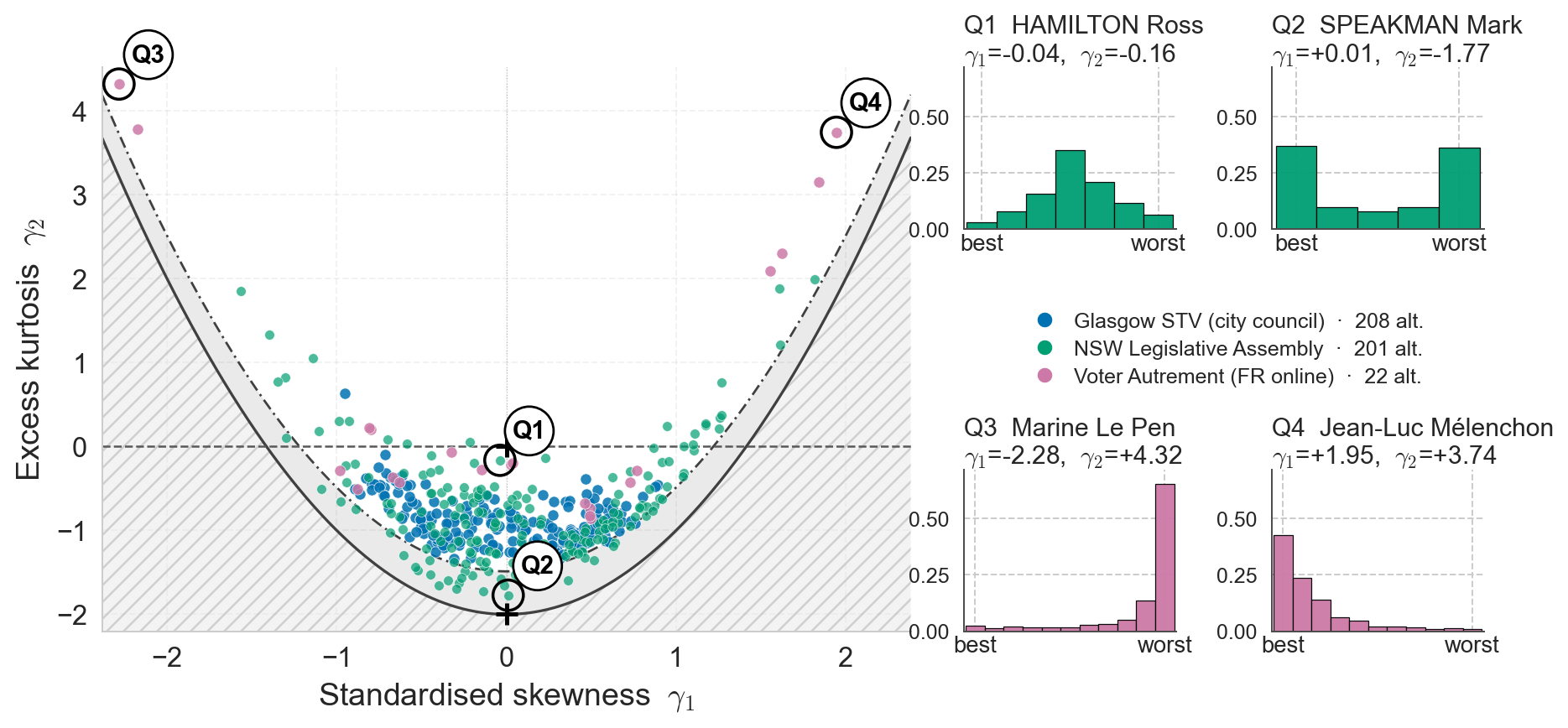
The same plane — real elections

Original real-election moment-plane figure

Complete-ranking ballots · Glasgow STV · NSW LA · French presidential

Technical branch · real elections

The empirical figure illustrates diversity, not an impossibility result

  • Observation unit: one candidate in one complete-ranking election.
  • Rank scales are normalized before comparing datasets with different numbers of alternatives.
  • Only complete-ranking ballots are retained.
  • This filter can over-represent more engaged voters.

The figure supports the claim that varied rank-distribution shapes occur in real data. Exact lower-degree indistinguishability is established by the synthetic witness, not by this plot.

The practical question

How much should we ask each person?

The target measure determines a required degree. The interface still has a choice about how to collect it.

λ
Maximum pairwise comparisons asked of one participant
N
Total participants required

Several comparisons with the same participant can reveal higher-degree information.

A chain of simple choices

A chain finds a favorite through simple choices

B→D→A→C

Three comparisons yield one favorite observation for each nested prefix — not a complete ranking.

Reusing a ranking

A ranking answers many subset questions at once

C≻A≻D≻B

4 triple observations from 1 participant — useful reuse, but not four independent voters.

Technical branch · elicitation primitives · 1/2

Query size, target degree, and dependence are different notions

  • A chain on k alternatives yields the favorite of each nested prefix.
  • A complete ranking on k alternatives implies the favorite of every subset.
  • At target degree 3, a ranking of exactly three alternatives and a 3-chain each yield one triple winner.
  • Reuse appears when a larger ranking covers several triples or several degrees.

Observations derived from one voter are dependent. Sampling guarantees concern repeated observations across appropriately sampled respondents.

Technical branch · elicitation primitives · 2/2

Naive pooling can change what is being estimated

If longer chains are shown only to unusually engaged participants, inferred comparisons from those chains need not represent the same population as short-query answers.

Within voter

Transitivity permits logical reuse.

Across voters

The sampling design must preserve the target population.

The lower-bound scope must match the query model; finding one person’s favorite does not automatically lower-bound every population estimator.

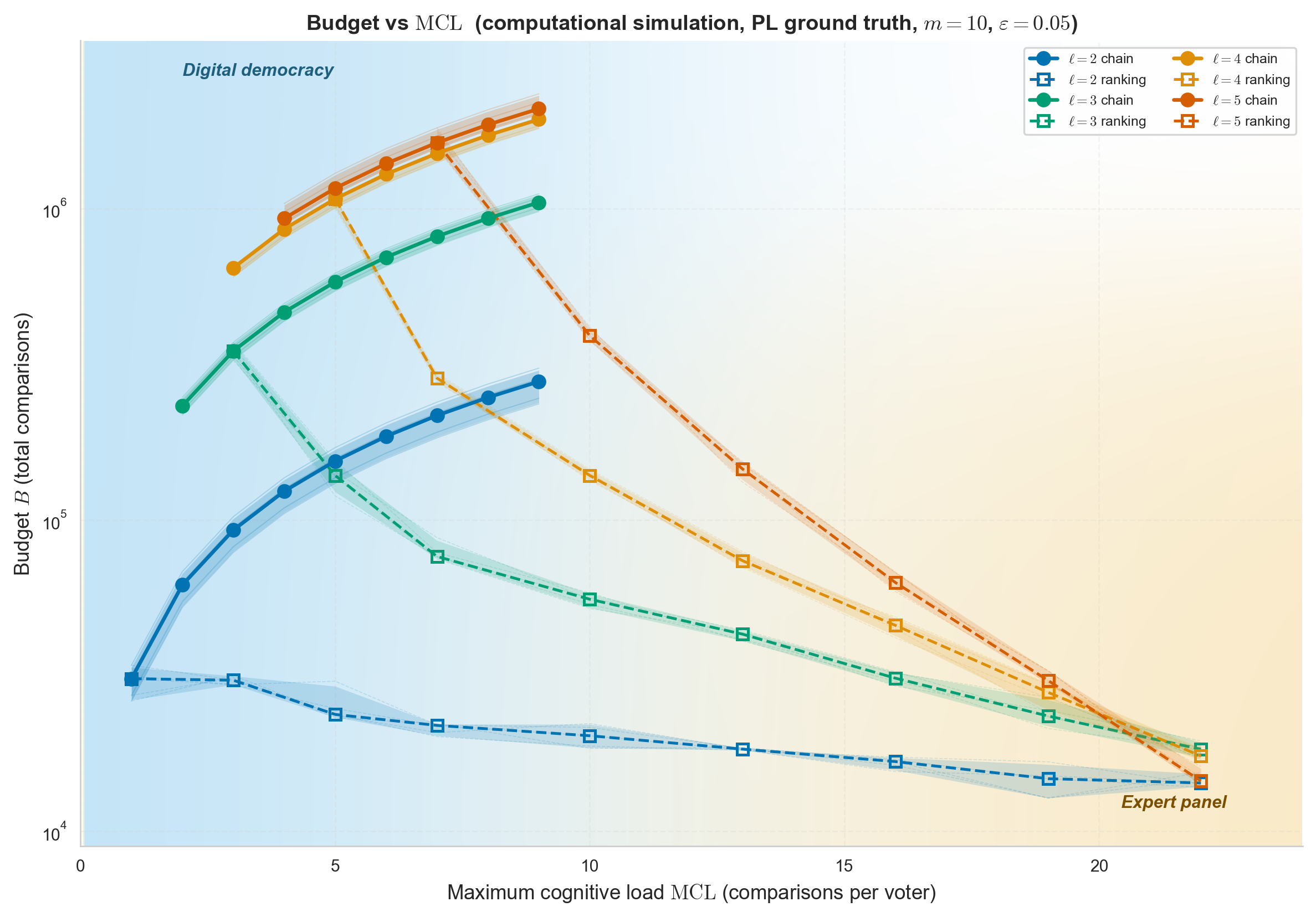
The elicitation frontier — effort and population

Original elicitation frontier figure

Richer answers can reduce the number of participants. Chain ● · ranking ▢

Technical branch · effort and population · 1/2

A fixed entry gets a finite-sample guarantee first

$$\Pr\!\left(|\widehat p-p|\ge\varepsilon\right)\le 2e^{-2n\varepsilon^2}.$$

Then a union bound covers all requested entries, provided each receives enough appropriately sampled observations.

  • Within-voter correlations do not invalidate the union bound.
  • Repeated observations of one entry need the stated sampling guarantee across respondents.
  • Entrywise error is not automatically the same error for a nonlinear disagreement score.

Technical branch · effort and population · 2/2

Read the experimental frontier within its scope

  • Ten alternatives and entrywise accuracy target \(\varepsilon=0.05\).
  • Filled circles: chains. Open squares: rankings.
  • Population is total comparison budget divided by per-voter load for each homogeneous protocol.
  • The source experiments report 5–95% quantiles across experimental seeds.

The plotted frontier compares the evaluated protocols; it does not prove global optimality over all elicitation strategies.

The design principle

The question determines the information to collect

1 · Question
Understand variation in candidates’ ranks
→
2 · Information
Pairs and triples are sufficient for rank variance
→
3 · Protocol
Choose chains or rankings to fit participants’ available effort

Understanding disagreement starts with knowing which information to ask for.

EDDY 2026

Thank you

Questions welcome.

ouaguenouni.com